Input panel

The input panel provides the options to specify the functionality, materials and their properties, polarimetry settings, etc. Each subpanel in the input panel can be expanded or collapsed as required by clicking on the arrow in the upper left corner.

Functionality

This subpanel allows the user to provide the material properties and choose what to calculate.

• The User Guide is selected by default when the notebook is evaluated. It displays the Welcome Page and a quick example of how to use ♯SHAARP.ml on the output panel.

• The Set Material Properties tab allows the user to describe the multilayer to be probed by specifying the materials, thicknesses, crystal structures and orientations and their optical properties (linear and non-linear susceptibilities).

• SHG Simulation shows the polarimetry settings to simulate the SHG intensities for the given multilayer. It also provides the options to display the Fresnel coefficients and Maker Fringes plot, and apply various assumptions as required.

• The 2D(3D) Schematics (available only when SHG Simulation or Set Material Properties is selected) shows the multilayer in real space as an interactive 2D(3D) figure on the output panel.

• Partial Analytical Expressions derives the SHG reflectance and transmittance in terms of unknown layer thicknesses and SHG tensor elements provided as symbolic variables in the Set Material Properties tab.

Set Material Properties

The following sub-panels are visible when the Set Material Properties tab is selected in the Functionality sub-panel.

Wavelength Setting

• Enter the wavelength (in vacuum) of the fundamental light incident on the multilayer.
• The value is to be entered in $\mu$m.

Layer Selection

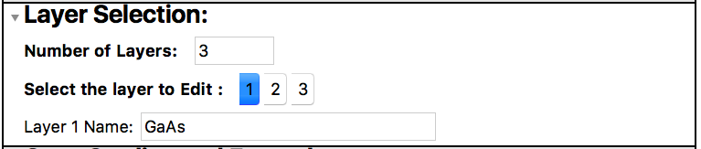
• Number of Layers refers to the number of layers that the multilayer is made up of.
• Each layer can be assigned a name by the user in the text box provided.
• Select the layer number whose properties need to be modified.

Case Study and Examples

• Crystal and optical properties of some common materials such as air, LiNbO₃ (LNO), KTiOPO₄ (KTP), etc. are pre-defined for convenience. The user may just click the layer number and select any of the above to quickly apply the properties to the selected layer.
• Click on Blank linear or Blank nonlinear to define a new linear or non-linear material with user provided crystal structure, crystal orientation, linear susceptibilities (and SHG tensors for non-linear materials).

Layer thickness

• Set the layer thickness in $\mu$m.
• In case of partial analytical expressions, click on analytical h to assign the layer i an unknown thickness (hi by default) where i is the layer number selected in the Materials Selection sub-panel.

Crystal Structure

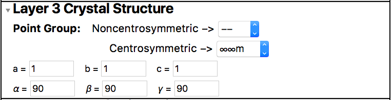
• Select the point group of the ith layer from the drop-down menu.
• Enter the crystallographic constants describing the unit cell. The lengths $a$, $b$, $c$ are to be entered in Angstroms and the bond angles $\alpha$, $\beta$, $\gamma$ in degrees.

Crystal Orientation

To define the crystal orientation of the selected layer, one can use either the Miller Indices (hkl) or the Crystal Physics Directions.

• In case of Miller Indices (hkl), the first set of h-k-l values corresponds to the respective surface plane (hkl) while the next set of h-k-l defines the direction perpendicular to the plane of incidence [hkl].

• If using Crystal Physics Directions, enter the components of the vectors $Z_1$, $Z_2$, $Z_3$ in the lab coordinate system $(L_1, L_2, L_3)$.

Click Update to visualize the crystal orientation of the selected layer with respect to the lab coordinate system on the output panel as a 2D/3D schematic.

Dielectric tensors

• Enter the dimensionless dielectric tensor $\epsilon_{ij}$ (as expressed in the crystal physics coordinate system) at both, the fundamental $\omega$ and the second-harmonic $2 \omega$ frequencies.
• Note that complex values may be entered above. Mathematica® uses I (capital i) to denote iota, the complex second root of unity.
• For the materials in the Case Study sub-panel, the dielectric tensor at $\omega$ and $2 \omega$ frequencies are set to update with the fundamental wavelength provided by the user. For this to work, the user needs to enter the wavelength first and then select the material from the Case Study sub-panel.

SHG tensor

• Enter the components of the SHG tensor $d_{ij}$ (expressed in Voigt notation) in units of pm/V​. Note that constraints due to the point group symmetry are automatically imposed on the SHG tensor.
• Click analytical dij if interested in partial analytical expressions involving unknown SHG tensor components. The components are labelled as dijmk by default (here, k refers to the layer number). The values are assumed to be in units of pm/V.
• In the case where certain components of the SHG tensor is known, click analytical dij and manually enter the known components. In this case, the partial analytical expression only involves the unknown symbolic components.

Layer Properties Preset Values

Apart from the already provided presets in the case study sub-panel, the user may define the film thickness, crystal structure, orientation, dielectric tensors (at fundamental and second harmonic frequencies) and SHG tensors for a material of their choice and save it as a preset.

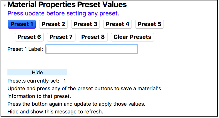
To save a preset, first enter the crystal and optical properties of the layer. Click Update and then select the Preset 1 to save the values. Similarly, one needs to save the properties to the other presets. When a preset is saved, the corresponding button appears blue.

To apply the preset values, first select the layer from the material selection sub-panel and then click the Preset i button to apply the properties stored in the i preset to the selected layer. Clear Presets removes all the saved preset information.

SHG Simulation

The following sub-panels describe the required parameters for generating the polar plots, Fresnel coefficients and Maker fringes.

Calculation Controls

Check if a plot of Fresnel coefficients and/or Maker fringes as a function of incident angle is to be generated.

Assumptions

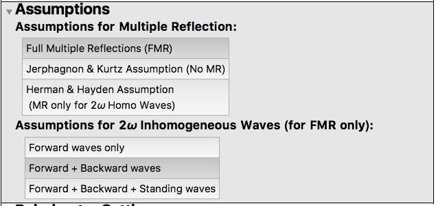
Click the respective boxes to apply full multiple reflections, Jerphagnon-Kurtz or Herman-Hayden assumptions for the calculation of the polar plots, Fresnel coefficients and/or Maker fringes. In case of full multiple reflections, further specify if backward waves need to be considered, and if so, whether to consider standing waves or not.

Polarimetry Settings

• Incident angle $\theta^i$ specifies the angle (in degree) between the incident ray and the normal to the incident surface. The user may either manually enter a value between 0$^{\circ}$ and 90$^{\circ}$ in the box, or use the slider to set the required value. Some commonly used angles are also provided; click the respective angle to set it.
• The incident electric field vector may be characterized by the polarization angle $\varphi$ and the ellipticity $\Delta \delta$ (both in degrees).
• The ellipticity $\Delta \delta$ may be manually set by entering a value (in degree) between 0$^{\circ}$ and 360$^{\circ}$ in the provided box or by dragging the slider.
• Depending on the measurement setup, one may choose either a rotating polarizer or a fixed polarizer. In case of the latter, the polarization angle $\varphi$ (in degree) may be entered by providing a value between 0$^{\circ}$ and 360$^{\circ}$ in the box, or by dragging the slider. Some commonly used angles are also provided.
• $\varphi=0^{\circ}$ corresponds to p polarized light while $\varphi = 90^{\circ}$ corresponds to s polarization. With respect to the lab coordinate system, $\varphi=90^{\circ}$ points in the direction of $+L_2$.
• Similarly, either a rotating analyzer or a fixed analyzer setting may be used depending on the optical setup. The angle, if required, is set similar to as described above.
• For a rotating polarizer, rotating analyzer setup, the analyzer-polarizer offset angle may be entered (in degree).

Fresnel coefficients collection settings

The Fresnel coefficients are calculated for incident angles $\theta^i$ from 0$^{\circ}$ to 90$^{\circ}$. The step size (in degree) determines the resolution of the calculated plot. A smaller step size produces a finer plot but takes longer time for the calculation.

Maker Fringes collection settings

Note: This sub-panel is visible only if Generate Maker Fringes Plot is checked in the Calculation Controls sub-panel.

• The Maker fringes are calculated for incident angles $\theta^i$ lying between $\theta^{min}$ and $\theta^{max}$. As described previously, provide the required values for $\theta^{min}$ and $\theta^{max}$ (in degree).
• Set the scan step size (in degree) depending on the required accuracy.
• As described in the Polarimetry Settings sub-panel above, enter the incident polarization angle, analyzer angle and the ellipticity (all in degree).

Partial Analytical Expressions

• Select the assumptions to be applied while solving for the reflection and transmission coefficients from the Assumptions sub-panel.
• In the Polarimetry Settings sub-panel, enter the incident angle and ellipticity in degree. Depending on the requirement, the polarizer and analyzer angles may be entered. See Polarimetry Settings under SHG Simulation for more details.